Spectral Clustering
Why Spectral Clustering
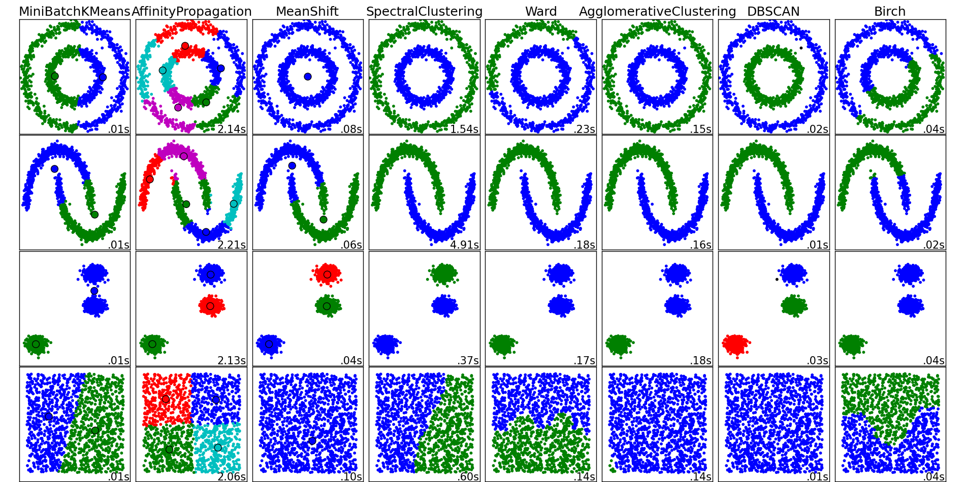
K-mean is a very popular clustering algorithm. It is very fast to train (O(n)), and it often gives reasonable results if the clusters are in separated convex shapes. However, if the clusters are connected in a different form, for example the inner circle and outer circle as seen in the image below, K-Mean will have trouble learning the cluster.
This is the case because the way the loss function of K-Mean is defined. It attempts to minimize the sum of distance between all points to a center. It is global in a sense. Spectral Clustering is different in that aspect, it only try to minimize the distance between a point and its closest neighbors. So within a cluster, for example the circle shape, two points can be very far away, but as long as there is a sequence of points with in that cluster that connect them, then that is fine.
So Spectral Clustering will work well with clusters that are connected, but can have any shape (does not have to be convex).
The Vanilla Spectral Clustering
The Spectral Clustering is as followed: given a dataset \( X \in \mathbb{R} ^ {n \times p}\)
-
Compute the affinity matrix This has the effect of focusing on small distance, and making all big distance equal to 0. It emphasize local, connectedness. This matrix is symmetric.
-
Construct degree matrix
-
Construct Laplacian matrix This matrix is symmetric, PSD
-
Find \(m\) smallest eigenvalues and associated eigenvectors (possibly ignoring the first). Let \(V \in \mathbb{R} ^ {n \times k}\) be the matrix containing the vector as columns
-
Performing k-Means on V. The cluster obtained from here is the result.
Variants
Following are some popular variants of the spectral clustering algorithm. Each variant has a different computational or theoretical aspect.
- Affinity Matrix: all of these affinity matrix try to make the
- The version we use is a fully connected version using Gaussian kernel transform. It is fully connected because even though the distance which are far away is very close to zero, it is still non-zero.
- \(\epsilon \)-neighborhood: make a graph where two points are connected if distance is less than \( \epsilon \). This in effect is a hard threshold version of the Gaussian kernel. This is a sparse matrix, and is computationally cheaper than the fully connected version.
- k-NN graph: two points ((i,j)) are connected if ((i)) is in ((k))-NN of ((j)) and vice versa. This is also a sparse matrix.
- Graph Laplacian
- Unnormalized: \( L = D - A \)
- Normalized \( L = I - D ^ {-1/2} A D ^ {-1/2}\)
- Normalized \( L = I - D ^ {-1} A\)
Properties
- Spectral Clustering emphasize connectedness, close neighbor distances, while ignoring faraway observations. It is then a local method (not global like K-Means).
- It is \( O(n ^ 3)\) in general and can be reduced to \( O(n ^ 2)\). In practice it is quite slow with large dataset (i.e. > 5000 observations). One should use the sparse version of affinity matrix.
- There are many theoretical results on Spectral Clustering
- Sensitive w.r.t. similarity graph
- Choose \( k \) the number of cluster such that \( \lambda_1, …, \lambda_k \) are small while \( \lambda_{k+1} \) is relatively large, i.e. there is a gape.
- What Laplacian to use: if degree are similar, then they are all the same. If degree are spread out, then use \(L=I-D ^ {-1}W\) is recommended.
- Consistency issues: the unnormalized might converge to trivial solution (1 point vs rest), or fail to converge as \( n\rightarrow\infty.\) Both normalized version converge under mild condition. To avoid trivial solution, make sure \( \lambda_{k}\ll\min d_{j}.\)
Reference
- Ulrike von Luxburg. A Tutorial on Spectral Clustering.
- Donghui Yan, Ling Huang, Michael I. Jordan. Fast Approximate Spectral Clustering.
- Trevor Hastie, Rob Tibshirani, Jerome Friedman. Element of Statistical Learning.