Decision Trees, Random Forest, Gradient Boosting
1. Decision Tree
1.1. Intro
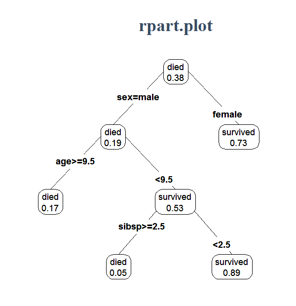
Decision trees sound straightforward enough, as for example seen in Figure 1. It is however not that straightforward to implement. We try to do it here.
1.2. Algorithm
Assuming we are doing classification, \(y \in {0,1} ^ n\), and \(X \in \mathbb{R} ^ {n \times d}\)
A decision tree starts as follow:
-
For each of the d features in X, rank \( X _ i\) and sort the y according to that feature \( X _ i\). First calculate the Gini score for the sorted y, which is for \(p\) is the proportion of 1 in \(y \). Now we calculate the two Gini score for each of the \(n - 1\) possible splits. As follow for here \(p _ {i1}\) is the proportion of 1 in y_sorted[:i], and \(p _ {i2}\) is the proportion of 1 in y_sorted[i:], using numpy notation. Subtracting these \(n - 1\) Gini score by the total Gini score to get the information gain for each of the split. At the end, we have the best information gain out of all possible \( d(n - 1)\) splits. We pick the best split and move one to the next step.
-
In this second steps, we have two nodes, each with \(n _ 1, n _ 2\) observations respectively. For each nodes, we proceed as in Step 1 and split according to the best out of \(d (n _ i - 1) \) splits, for \(i \in \{1, 2 \}\).
-
We keep the same procedure until some pre-specified max depth, for example 8.
For regression, instead of using Gini coefficient, we use the Variance. Overall, the Gini coefficient and variance measure the purity of a node. These scores are small if all observations within the nodes are very similar to each other, and big if the observations are very different from each other. A decision tree wants this because it will classify all observation in each node to be the majority class, or in case of regression predicting all observation to be the mean.
1.3. Computation Complexity
For step 1, for each feature, getting the \(n - 1\) Gini coefficient is \(O(n) \). Sorting the feature is \( O(n\log n)\). So the total cost is \(O( nd \log n)\). We proceed this step 1 until some max depth. The max depth is in the order of \( O (\log n)\). So in total, the complexity should be \( O (nd (\log n) ^ 2)\). Overall, it is pretty efficient. Note that for some variant, we don’t consider all \(d\) feature at each split, but only a portion, this might reduce the complexity a bit further.
The codes to get the \(n - 1\) Gini score efficiently in \(O(n)\) is as followed.
from __future__ import division
import numpy as np

def GetP(y):
    """ This function return the proportion of 1 in y[:i],
	for i from 1 to length(y)
    Parameters:
    -----------
        y: numpy binary 1D array
    Returns:
    --------
        numpy float 1D array of length n - 1, containing proportion of 1
    """
    n = len(y)
    return (y.cumsum()[:-1] / np.arange(1,n))

def GetGini(y):
    """ Return the Gini score of y for each way of splitting,
        i.e. Gini( y[:1], y[1:] ), Gini(y[:2], y[2:], ...)
    """
    n = len(y)
    p1 = GetP(y)
    p2 = GetP(y[::-1])[::-1]
    res = np.arange(1,n) * p1*(1 - p1) + np.arange(1,n)[::-1] * p2 * (1 - p2)
    return res / n
1.4. Hyper Parameters
For a tree, the important hyperparameters control its complexity
- Max Depth: the lower it is, the less complex. It should not be much higher than \( \log _ 2 n \)
- Min Sample Nodes: each node should contain at least this many samples
- Min Sample split: to consider split a node, the node must have at least this many samples (note that this is different from 2.)
- Max number of nodes: this is straight forward, and is roughly equal to \(2 ^ {maxdepth}\).
- Criterion: for classification, in addition to Gini score, one can use entropy, which is \(p \log p + (1 - p) \log (1 - p)\). The two functions are in fact very similar
2. Ensembles
2.1. Random Forest
Once we understand decision tree, random forest is a piece of cake. It basically do
- Sample \(\alpha n, \alpha \in [0,1]\) observations from the original dataset, and \(\beta p, \beta \in [0,1]\) features, and build a tree here
- Repeat the process for k times, and classify observations according to majority, or regression observation according to the mean.
Three more hyper parameters that we introduced:
- Proportion of observation to sample: the smaller it is, the more independent the different trees are
- Proportion of feature to sample: similar to 1. For classification, it is recommended to be around \(\sqrt{d}\), for regression, it is recommended to be \(d / 3\)
- Number of trees: basically the bigger the better, but just more computation.
Each of the trees in Random Forest is independent of each other, and thus can be embarrassingly paralleled. In general, the technique of averaging many small models, where each model use a bootstrap sample of the data, is called bagging (bootstrap aggregation).
2.2. Gradient Boosting Machine
The algorithm is as followed (credit ESL)
- Initialize \(f _ 0 (x) = \arg \min _ {\gamma} \sum _ {i = 1} L(y _ i, \gamma) \)
- For m = 1 to M:
- For \(i = 1, 2, …, N\) compute
- Fit a regression tree to the target \(r _ {im}\) giving terminal regions \(R _ {jm}, j = 1, 2, …, J _ m.\)
- For \(j = 1, 2, …, J _ m\) compute
- Update \( f _ m (x) = f _ {m - 1} (x) + \sum _ {j = 1} ^ {J _ m} \gamma _ {jm} I(x \in R _ {jm})\)
- Output \(\hat{f} (x) = f _ M (x).\)
For regression with loss function \(L(y, \gamma) = (y - \gamma) ^ 2\), we have
- Initialize \(f _ 0 (x) = \bar{y} \)
- For m = 1 to M:
- For \(i = 1, 2, …, N\) compute
- Fit a regression tree to the target \(r _ {im}\) giving terminal regions \(R _ {jm}, j = 1, 2, …, J _ m.\)
- For \(j = 1, 2, …, J _ m\) compute , for \(\bar{y} _ {jm}\) is the mean of \(y\) in that region
- Update \( f _ m (x) = f _ {m - 1} (x) + \sum _ {j = 1} ^ {J _ m} \gamma _ {jm} I(x \in R _ {jm})\)
- Output \(\hat{f} (x) = f _ M (x).\)
Basically, we start with a simple regression tree, and calculate the residual. We then fit a model to the residual, and calculate the aggregated model. We calculate the new residual and keep proceeding. For classification, the deviance loss function can be used.
Some improvements
- Use shrinkage in Step 2.4. The update rule is \( f _ m (x) = f _ {m - 1} (x) + \nu \sum _ {j = 1} ^ {J _ m} \gamma _ {jm} I(x \in R _ {jm})\), for \(\nu \in (0, 1]\). This is similar to a learning rate. Lower learning rate needs more iteration (more trees)
- Subsample observations, and columns
For hyperparameters, in addition to the 3 hyperparameters as found in Random Forest, Gradient Boosting Machine has 1 additional important hyperparameter which is learning rate. Typically, lower learning rate is better for testing error, but should be accompanied with more trees.
Unlike Random Forest, Gradient Boosting is not easily paralleled. It is still however still doable at each step. More specifically one can use multiple cores to speed up the building of each tree. In some sense Gradient Boosting is similar to Neural Network training with gradient descent. There is both a learning rate, and early stopping. It is not parallelizable along the iteration, but each iteration can be parallelized.
Gradient Boosting is also similar to Stagewise Regression, in that it fits to the residual iteratively at each step.
3. Implementations
In R, decision tree is implemented in rpart, while in Python, one can use scikit-klearn. Since we rarely use decision tree, but more often the ensembles, we talk about these more here. Random Forest and Gradient Boosting have their official packages built by the original algorithm of the inventor in R (Leo Breiman and Jerome Friedman). These two packages have a lot of parameters to tweak; however, they are slow and only use 1 core.
In Python, RandomForest of Scikit-Learn is fast and uses multiple core. GBM is slow here however. In both R and Python, one can use XGBoost to run Random Forest and GBM really fast and on multiple cores. The algorithm in XGBoost is actually slightly different than GBM. According to the author
Both xgboost and gbm follows the principle of gradient boosting. There are however, the difference in modeling details. Specifically, xgboost used a regularized model formalization to control over-fitting, which gives it better performance.
To be specific, the loss function is added with an L2 term \( \frac{1}{2} \lambda \sum _ {j = 1} ^ T w _ j ^ 2\), where \(w _ j\) is the tree prediction for each leaf. XGBoost is very popular among Kaggle competitors. It is in many of the winning solutions, and can also be used to run Random Forest. In fact, one can have a hybrid of both Random Forest and Gradient Boosting, in that we grow multiple boosted model and averaging them at the end.
Finally, Scikit-learn has an implementation of Extra Trees (also called Extremely Randomized Trees). Instead of using the best split for each feature, it uses a random split for each feature. This allows the variance to be reduced, and quite often performs better than Random Forest.
In R, H2O also provide fast implementation of Random Forest and Gradient Boosting.
References and Credits
- Element of Statistical Learning
- Tianqi Chen (Author of XGBoost)
- Leo Breiman (Author of CART, Random Forest)
- Jerome Friedman (Author of CART, GBM)